Page 10 - revista Ingeniantes 4 No1 Vol 1 Interectivo
P. 10
Revista Ingeniantes 2017 Año 4 No. 1 Vol. 1

Then, using the matrix table showed above, the corre-           Table 3: Standardized data
lation coefficient was estimated for each item. The
results of the analysis are shown below:                        Item 1 STD Item 1 STD_1Item 1 STD_2Item 1 STD_3Item 1 STD_4Item 1 STD_5Item 1 STD_6Item 1 STD_7Item 1 STD_8Item 1 STD_9Item 1 STD_10Item 1 STD_11

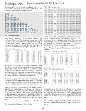
Fig. 1: Correlation Matrix                                      -1.63897056 0.1080945 -1.28846231    0 -0.56785207 -1.84816895 -1.59128698 -0.85080176 -2.54471863 -1.50143244 -1.34363195 -1.97708056

The figure 1 presents the correlation between the               -1.63897056 0.1080945 -0.06135535    0 -0.56785207 -0.24106552 -1.59128698 -2.06623285 -1.11107433 0.31848567 0.3900867 -0.29445881
analyzed items and the obtained responses in the
number of the questionnaires applied. According to              -0.18210784 0.1080945 -0.06135535 -1.22474487 1.17938506 1.36603792 0.08375195 1.58006041 0.32256997 -1.50143244 0.3900867 1.38816295
the correlation matrix, it was obtained that there is an
adequate correlation by items, due this, the expected           -0.18210784 -1.33316549 -0.06135535 -1.22474487 1.17938506 -0.24106552 0.08375195 0.36462933 0.32256997 -1.50143244 -1.34363195 -0.29445881
values of correlation must be higher than the 0.70.
                                                                -0.18210784 0.1080945 -0.06135535    0 1.17938506 -0.24106552 0.08375195 0.36462933 1.75621426 2.13840377 2.12380534 -0.29445881
Table 2: Cronbach Alpha
                                                                -0.18210784 -1.33316549 -0.06135535 1.22474487 1.17938506 1.36603792 0.08375195 -0.85080176 0.32256997 -1.50143244 -1.34363195 -0.29445881

                                                                -0.18210784 0.1080945 -1.28846231    0 1.17938506 -0.24106552 -1.59128698 0.36462933 0.32256997 -1.50143244 2.12380534 -0.29445881

                                                                -0.18210784 0.1080945 -1.28846231    0 1.17938506 -0.24106552 -1.59128698 0.36462933 0.32256997 0.31848567 0.3900867 -0.29445881

                                                                -0.18210784 0.1080945 -0.06135535    0 1.17938506 -0.24106552 0.08375195 1.58006041 1.75621426 0.31848567 0.3900867 -0.29445881

                                                                -1.63897056 0.1080945 -1.28846231    0 1.17938506 -0.24106552 0.08375195 -0.85080176 1.75621426 2.13840377 0.3900867 1.38816295

                                                                -3.09583328 -2.77442548 -1.28846231  0 -0.56785207 -1.84816895 0.08375195 -0.85080176 -1.11107433 0.31848567 -1.34363195 -0.29445881

                                                                -0.18210784 0.1080945 -1.28846231 -1.22474487 -0.56785207 1.36603792 -1.59128698 0.36462933 0.32256997 0.31848567 -1.34363195 -0.29445881

                                                                -0.18210784 1.54935449 1.16575162    0 -0.56785207 1.36603792 1.75879087 0.36462933 1.75621426 0.31848567 0.3900867 -0.29445881

                                                                -0.18210784 -1.33316549 -2.51556928 -2.44948974 -0.56785207 -1.84816895 0.08375195 -0.85080176 -1.11107433 -1.50143244 -1.34363195 -0.29445881

                                                                -0.18210784 0.1080945 1.16575162     0 -0.56785207 -0.24106552 1.75879087 0.36462933 0.32256997 0.31848567 0.3900867 -1.97708056

                                                                1.27475488 0.1080945 1.16575162 1.22474487 -0.56785207 -0.24106552 1.75879087 1.58006041 1.75621426 0.31848567 0.3900867 1.38816295

                                                                -0.18210784 0.1080945 1.16575162 1.22474487 -0.56785207 -0.24106552 -1.59128698 -0.85080176 0.32256997 0.31848567 0.3900867 1.38816295

                                                                -0.18210784 0.1080945 -0.06135535    0 1.17938506 1.36603792 0.08375195 1.58006041 0.32256997 0.31848567 0.3900867 -0.29445881

                                                                1.27475488 0.1080945 -0.06135535 1.22474487 1.17938506 1.36603792 0.08375195 -0.85080176 0.32256997 0.31848567 0.3900867 -0.29445881

                                                                -1.63897056 0.1080945 -1.28846231    0 -0.56785207 1.36603792 0.08375195 -0.85080176 -1.11107433 0.31848567 2.12380534 -1.97708056

                                                                1.27475488 0.1080945 1.16575162      0 1.17938506 -0.24106552 0.08375195 0.36462933 0.32256997 0.31848567 0.3900867 -0.29445881

                                                                -0.18210784 -1.33316549 -0.06135535  0 -0.56785207 -0.24106552 0.08375195 -0.85080176 -1.11107433 0.31848567 0.3900867 -0.29445881

                                                                -0.18210784 0.1080945 -0.06135535 -1.22474487 -0.56785207 -0.24106552 -1.59128698 0.36462933 -1.11107433 0.31848567 -1.34363195 -0.29445881

                                                                -0.18210784 -1.33316549 -1.28846231 -2.44948974 -0.56785207 -0.24106552 0.08375195 -2.06623285 -1.11107433 -1.50143244 -1.34363195 -1.97708056

                                                                -0.18210784 0.1080945 1.16575162 -1.22474487 -0.56785207 1.36603792 0.08375195 -0.85080176 -1.11107433 0.31848567 0.3900867 -0.29445881

                                                                -0.18210784 0.1080945 1.16575162     0 -0.56785207 -0.24106552 0.08375195 1.58006041 0.32256997 2.13840377 0.3900867 1.38816295

                                                                -0.18210784 0.1080945 1.16575162 1.22474487 1.17938506 1.36603792 0.08375195 1.58006041 0.32256997 0.31848567 0.3900867 1.38816295

                                                                -0.18210784 0.1080945 1.16575162     0 1.17938506 -0.24106552 1.75879087 0.36462933 0.32256997 0.31848567 0.3900867 1.38816295

                                                                -0.18210784 0.1080945 1.16575162     0 1.17938506 -0.24106552 1.75879087 -0.85080176 0.32256997 -1.50143244 -1.34363195 1.38816295

                                                                -0.18210784 -1.33316549 -0.06135535 1.22474487 -0.56785207 -0.24106552 0.08375195 -0.85080176 -1.11107433 0.31848567 0.3900867 -0.29445881

                                                                1.27475488 -1.33316549 -0.06135535   0 -2.31508919 -1.84816895 0.08375195 0.36462933 0.32256997 0.31848567 0.3900867 -0.29445881

                                                                1.27475488 0.1080945 -0.06135535     0 -0.56785207 -0.24106552 1.75879087 -0.85080176 0.32256997 -1.50143244 -1.34363195 1.38816295

                                                                -0.18210784 -1.33316549 -0.06135535 -1.22474487 -0.56785207 1.36603792 0.08375195 0.36462933 -1.11107433 0.31848567 0.3900867 -0.29445881

                                                                1.27475488 0.1080945 -0.06135535 1.22474487 -0.56785207 1.36603792 0.08375195 0.36462933 0.32256997 0.31848567 0.3900867 -0.29445881

                                                                1.27475488 1.54935449 -0.06135535 1.22474487 -0.56785207 -0.24106552 0.08375195 0.36462933 0.32256997 0.31848567 -1.34363195 -0.29445881

                                                                1.27475488 1.54935449 1.16575162 1.22474487 -0.56785207 -0.24106552 0.08375195 1.58006041 0.32256997 0.31848567 0.3900867 1.38816295

                                                                1.27475488 1.54935449 1.16575162     0 -0.56785207 -0.24106552 0.08375195 0.36462933 0.32256997 0.31848567 0.3900867 -0.29445881

                                                                -0.18210784 1.54935449 -0.06135535 1.22474487 -0.56785207 -0.24106552 0.08375195 -0.85080176 -1.11107433 0.31848567 0.3900867 1.38816295

                                                                1.27475488 1.54935449 -1.28846231 -1.22474487 -2.31508919 -1.84816895 -1.59128698 -0.85080176 -1.11107433 -1.50143244 -1.34363195 -0.29445881

                                                                1.27475488 1.54935449 1.16575162 1.22474487 1.17938506 -0.24106552 0.08375195 0.36462933 0.32256997 0.31848567 0.3900867 -0.29445881

                                                                On the other hand, once applying the data standardiza-
                                                                tion as shown in Table 5, the significant factors of cus-
                                                                tomers are determined according to the 5 dimensions
                                                                established in section 6. Next the standardized data,
                                                                the Mahalanobis distance is estimated to determine
                                                                the significant items using Minitab 17 as shown:

                                                                Table 4: Principal Component Factor Analysis of the Correla-
                                                                tion Matrix

According to the results of Cronbach’s alpha for each           Table 5: Factor Score Coefficients
item ≥ 0.7 it is assumed that the applied questionnaire me-
asures the necessary dimensions of SERVPERF model
to estimate the quality of service. In addition Cronbach’s
alpha global, that is, the overall average of the coefficients
is equal to 0.8006 or 80.06% expressed as a percentage
indicating a good fit of the data to be measured.

Once the analysis of the Cronbach coefficient has been
accepted, and proving that the items measure the requi-
red dimensions, the data of each item were normalized in
order to establish the main factors, as shown below.

With the results of the coefficients, the data is standar-
dized to use the average μ and standard deviation σ as          As can be seen the dispersion of data on the effect
the parameters, in other words the data are normalized          of each item on the perception of quality is distribu-
to estimate the Mahalanobis distance. A standardization         ted equivalently, in other words, the 12 questions that
of data was performed to convert qualitative variables to       include the 5 dimensions of the model SERVPERF be
quantitative type, using Minitab 17, allowing the change of     addressed in order to ensure an optimal experience
parameters. The standardization of data was carried out         quality.
by:                                                             Once found the significant factors improvement strate-
       =    −       →  ((0,1)  Eq. (6)          gies were established according to each dimension ba-
                                                            sed on:

The standardized data table shown below:

                                                        06

