Page 59 - Ingeniantes 511 interactivo

Revista Ingeniantes 2018 Año 5 No. 1 Vol. 1

Hardware Description The function that computes the elementary criteria E as
The tests were made on connected computers in a a function of can be defined as a decreasing function
switch 3COM Ethernet with the next features: with the equation (1).
Server:
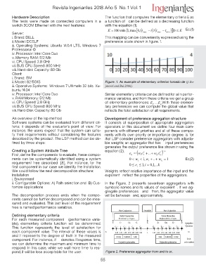
i. Brand: DELL E  100 min 1, max0,tmax  t/tmax  tmin 0  E  1E0c0.(%1)
ii. Model: DCSLF
iii. Operating Systems: Ubuntu 14.0.4 LTS, Windows 7 This mapping can be conveniently expressed using the
Professional © preference scale shown in figure. 1.
iv. Processor: Intel Core Duo
v. Memory RAM: 512 Mb Figure. 1. An example of elementary criterion tomado de (J. Du-
vi. CPU Speed: 2.8 GHz jmović and Bai 2006).
vii. BUS CPU Speed: 800 MHz
viii. Hard-disk Capacity: 80 Gb Similar elementary criteria can be defined for all n perfor-
Client: mance variables, and from these criteria we get a group
i. Brand: IBM toafryelpermeefenrteanrycepsrewfeerecnacnecso: mE1p,..u..tEen.tWheithgltohbeaslevaellueemtehna-t
ii. Model: 8215G1S reflects the total satisfaction of all requirements.
iii. Operative Systems: Windows 7 Ultimate 32 bits Xu-
buntu 14.04
iv. Processor: Intel Core Duo
v. RAM Memory: 512 Mb
vi. CPU Speed: 2.8 GHz
vii. BUS CPU Speed: 800 MHz
viii. Hard-Disk Capacity: 80 Gb

An overview of the lsp method Development of preference agregation structure
Software systems can be evaluated from different cri- It consists of superposition of appropriate aggregation
teria; it depends of the evaluator’s point of view. For operators. In this document we define four main com-
instance, the users expect that the system can satis- ponents with different priorities and all of these compo-
fy their requirements without considering the features nents with its own priority or importance degree. Is for
described by the product. The LSP method can be de- that LSP consider preference aggregators with adjusta-
fined by three steps: ble weights; an aggregator that has input preferences
Creating a System Atribute Tree generates the output preference like shown in using the
First, define the components to evaluate, these compo-
nents can be systematically identified using a system  equation (2). e0  w1e1r  ..  wk ekr 1/ r
requirement tree described [8].. For instance, for the
first component in our case we identify the Installation. 0  wi  1, w1  ..  wk  1 Ec(2)
We could follow the next decomposition structure:
Installation 0  ei  1,i  0,1,...k
i. Environment
ii. Configurable Options: A) Path selection and B) Cus- Weights reflect relative importance of the input and the
tomize applications exponent reflect the properties of the aggregators.
The decomposition process ends when the compo-
nents cannot be further decomposed and can be mea- In the Figure. 2 presents seventeen aggregators with
sured and evaluated. This last level of the requirement symbolic names and its values of exponent . If we ag-
tree is named performance variables. gregate preferences and then, the aggregator value
will be between and, approximately.

Defining elementary criteria Figure 2. Preference aggregator from and to or.
For each measured component (performance varia-
ble), elementary criteria function will be determined.
This function represents the level of satisfaction for
each component value. The interval of these values is
and it represents the degree of truth in the measured
component. For instance, if denotes Response time,
we can determine the maximum and minimum time to
respond. In this case, while we wait more time to res-
pond, it will be less acceptable for the user.

55